Quantifying class relationships by training DNN classifiers

In this post I will begin my explanation and exploration into the link between interpretable classification models and quantifying class traits/relationships.

To illustrate, I will use the class ImageNet1K dataset and a pretrained ResNet50 from the PyTorch model zoo:

from torchvision.models import resnet50

model = resnet50(weights=ResNet50_Weights.DEFAULT)

However, for the purposes of this post, we are actually only interested in the weights of the last layer:

last_layer_weights  = model.fc.weight.clone().detach()

# Apply some normalization
last_layer_weights -= last_layer_weights.mean(dim = 1, keepdim=True)
last_layer_weights /= last_layer_weights.std(dim = 1, keepdim=True)
# Save the magnitudes
last_layer_norm     = last_layer_weights.norm(2, dim=1)

The interesting thing about the last layer, is that it has a dimensionality of \(\{N_{classes}, N_{embeddings}\}\), since the output should be a (stack of) vector(s) containing the shifted log-probabilities for each class in the models repetoire. Another perspective may be gained by considering the scenario from the perspective of a single class, the shifted log-probability for that class is simply a dot product between the embeddings produced by the model backbone, and the corresponding row of weights in the last layer (+ the bias, here denoted \(k\)):

This looks awfully a lot like the formulation of a GLM (generalized linear model), leading to the intuition of the last layer as a stack of GLMs for each class. This would then lead to the not-so-suprising analogy that the embeddings are a set of a proxy-visual distinguishing characteristica between the classes (i.e. morphological traits). By combining these two insights, it becomes clear that the correlation structure between the values (or rather coefficients 😉) of the classes, contain information about the learned visual (morphological) similarity between classes.

Thus, a natural way to proceed is to use an appropriate distance/similarity function for vectors, and compute a pairwise distance/similarity matrix for further analyses. Here I will try out cosine similarity and euclidean distance, just because they are some of the most common metrics:

# Calculate pairwise cosine similarity
cos_mat  = (last_layer_weights @ last_layer_weights.T) 
cos_mat /= (last_layer_norm.unsqueeze(0) * last_layer_norm.unsqueeze(1))
# And euclidean distance
eucl_mat = torch.cdist(last_layer_weights, last_layer_weights)

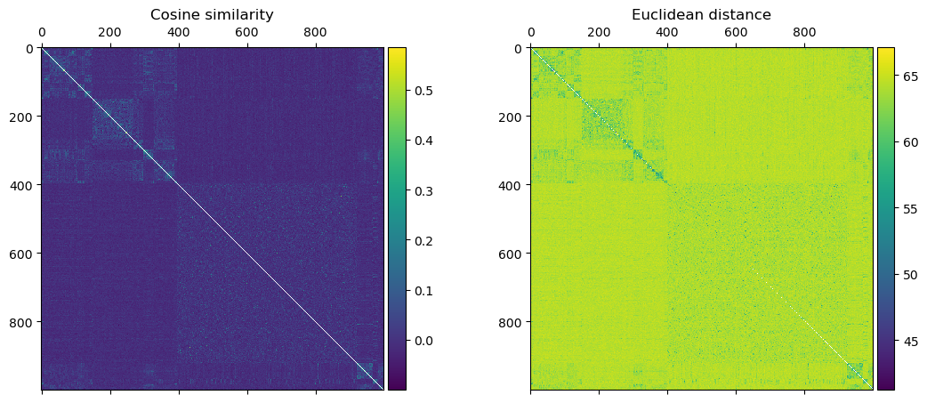
Which produces the following distance matrices:

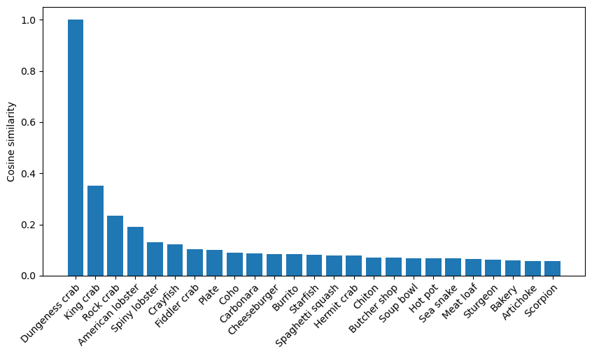
From which we can see clear signs of a defined learned structure in the weights. We can also take a look at a specific species — I have chosen the “Dungeness crab” — and look at the most similar classes:

focal_idx  = 118
focal_name = idx_to_name[focal_idx]

similar_classes, similarities = zip(*[
    [idx_to_name[i.item()], cos_mat[focal_idx, i].item()] 
    for i in cos_mat[focal_idx].argsort(descending=True)[:25]
])

Which produces the following:

Which again makes a lot of sense, first the other crabs in the ImageNet1K dataset, before moving to seafood, then food in general and then to unrelated classes (well as far as I can judge).

Lastly, we can also use the distance matrix for inference about the classes. For example, we can use classical hierarchical clustering methods:

from scipy.cluster.hierarchy import linkage, dendrogram

fdmat  = cos_mat[*torch.triu_indices(*cos_mat.shape, offset=1)]
fdmat  = (-cos_mat + 1) / 2
fdmat -= fdmat.min()
clust  = linkage(fdmat, "ward")

dendr  = dendrogram(
    clust, 
    labels=classes, 
    orientation="left", 
    color_threshold=2, 
    no_plot=True
)

Which produces the following:

If you look closely, you might find clusters such as “mushrooms” (small yellow group on the right-hand side) or “big game” (red group at the bottom).